Help for SwayStar™ (4.7.3.265)
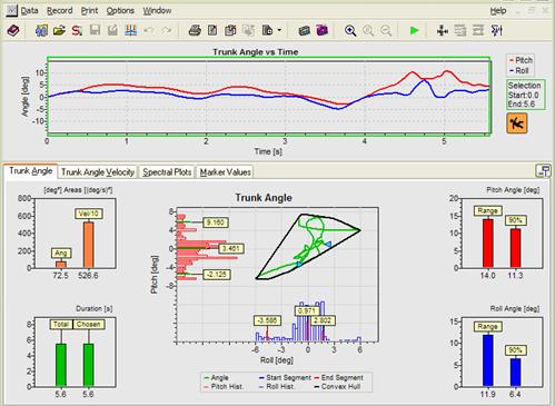
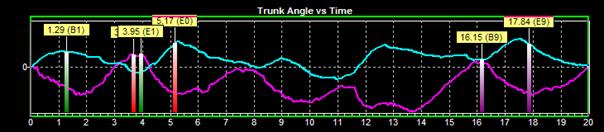
Angular deviations are calculated on-line using trapezoid integration of angular velocities recordings from the sensors, and are immediately available on re-analysis (for example, by changing the analysis time period of interest). The original recorded data can be retrieved at any time. The original sampled data can also be pasted into the Windows “Clipboard” for retrieval in Excel or Notepad. There are six analysis windows per recording: The original recordings as time plots, x-y plots of Trunk Angle and Trunk Angle Velocity, Spectral Plots of trunk angular velocity, Marker Values and finally analogue to digital (A/D) sampled values if simultaneous acquisition of analogue signals was performed (see section 2.10). In the case of a fall, if the subject lost balance the primary observation is the shortened task duration of the time plots and the loss of balance indicator, as well as large roll angle deviations as shown here:
Note: This patient starts (head of arrow pointing right in the trunk angle x-y plot) within the base of support (the orange octagonal shape shows the limits) and then falls to the right and forward after 5.6s (arrow pointing left). The fact that she lost balance is indicated by the orange fall indicator at the end of the recording.
If the subject did not loose balance then the fall indicator is green and the figure in the pictogram is standing. If data was recorded with earlier versions of SwayStar, the fall symbol contains a question mark.
All of the numerical values shown in the analysis windows plus a flag indicating loss of balance may be stored in an Excel (CSV) file.
PITCH
Range of peak-to-peak excursions: The extent of trunk pitch angular displacement over the complete trial.
90% range of pitch excursions: To define this range the peak-to-peak range of the subjects’ excursions is divided into 40 bins. Each sample of pitch angle taken every 10 ms is then assigned to one of these bins depending on its amplitude. With all samples binned, a histogram can be drawn shown in red to the left of the x-y amplitude plot in the above example. The 5% and 95% limits can be defined for the recording from this histogram. The amplitude between these limits is the 90% range.
Note: The 5%, 95% and median values of the subjects’ excursions, with respect to angular position at the start of the recording, are labelled on the histogram. The x-y (pitch-roll angle) plot is corrected to the median values (bias removed).
ROLL
Peak-to-peak roll excursions: The extent of trunk roll angular displacement over the complete trial.
90% range of roll excursions: The range is defined the same as for pitch, but in this case for roll (see blue histogram under the x-y amplitude plot).
Note: If more than 1 “spike artefact” occurs in the recording every 2 seconds on average, these spikes will have been removed and the data is then filtered. A filter symbol added is in the bar above the recording to indicate the presence of the correction for roll only. For this reason in the above display only the blue roll filter symbol is shown.
Sway area (angle) and mean path velocity
This is the area defined by the envelope of the pitch and roll excursions when these variables are plotted as an x-y plot (the convex hull). Mean path velocity (plotted in the velocity analysis window) is the mean velocity of the vector movement of roll and pitch angular displacements, sample to sample. As a reminder, the green arrows on the trunk angle and velocity x-y plots represent the start and stop positions of a subject.
Stability cone
This is shown by an orange line around the x-y angle plot. It indicates the maximum amount of sway young normals can achieve when leaning and maintaining a straight posture.
SAMPLED DATA
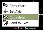 To paste the pre-processed
sampled streams of data into the Windows “Clipboard” place the mouse over
the trunk angle x-y plot (or angular velocity x-y plot) and simply choose
this option when the context dependent command box appears or right “click”
while holding down the “control” and “Shift” keys simultaneously. The
data is in tab-delimited form and has the following format:
To paste the pre-processed
sampled streams of data into the Windows “Clipboard” place the mouse over
the trunk angle x-y plot (or angular velocity x-y plot) and simply choose
this option when the context dependent command box appears or right “click”
while holding down the “control” and “Shift” keys simultaneously. The
data is in tab-delimited form and has the following format:
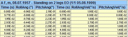
The list is headed by a line identifying the examination by the subjects name, first name, birth date and the name and date of the examination, followed by a header row identifying the data columns. Note that the sample interval is 10 ms.
PITCH
Range of peak-to-peak velocity excursions: The extent of trunk pitch angular velocity over the complete trial.
90% range of pitch velocity excursions: To define this range the peak-to-peak velocity range is divided into 40 bins. Each sample of pitch angular velocity is then assigned to one of these bins depending on its amplitude. With all samples binned a histogram can be drawn as shown in red to the left the x-y velocity plot in the above example. The 5% and 95% limits can be defined for the recording from this histogram. The velocity amplitude between these limits is the 90% range.
Note: The 5%, 95% and median values are labelled on the histogram. The x-y (pitch-roll angular velocity) plot is not corrected to the median values (no bias removal).
ROLL
Peak-to-peak velocity excursions: The extent of trunk roll angular velocity over the complete trial.
90% range of roll velocity excursions: This is defined in the same way as for pitch velocity but, in this case, for roll.
Sway area (angular velocity) and rms velocity
This is area-defined by the envelope of the pitch and roll velocity excursions when these are plotted as an x-y plot (the convex hull). Its value is listed in the angle window with values divided by 10. The root mean square (rms) velocity - plotted in the velocity analysis window is the square root of the squared mean velocity of the vector movement of roll and pitch angular displacements, sample to sample, with the mean velocity removed.
 Spectral densities
of pitch and roll angular velocities
Spectral densities
of pitch and roll angular velocities
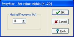
This is shown by the continuous curve in the diagram. The spectrum is computed using a moving box-car window of time period 2.56s with a shift of 0.64s from window to window. The spectra for all windows of the recording are averaged across the analysis period (green frame on time plots). The extent of the frequency axis can be changed in integer frequencies between 4 and 20 Hz using a right mouse button click.
Spectral weights
The columns in the diagram show these weights. They are computed by taking the spectral densities every 0.4 Hz computing the square root to get an estimate of the velocity amplitude at frequencies separated by 0.4 Hz and then averaged together at 3 values. That is, at 1.2 Hz the value is the average of 0.8, 1.2 and 1.6 Hz and so on for 2.4, 3.6, 4.8 Hz, etc.
Note: Spectral density values greater than 1 will lead to lower weights and, thus, values less than 1 higher weights.
Note: The copy function will copy either the Pitch Spectra or the Roll Spectra, depending on where the mouse pointer is resting.
The time period used for analysis can be reduced to less than the total recording time
by altering the analysis time-frame. This is the green frame shown in the example
below. The minimum analysis time is 1.26 s.
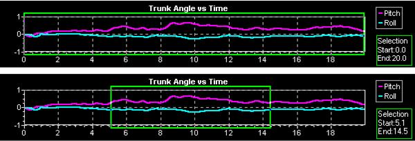
To change the analysis time (the
frame size), click within the graph, where you would like your selection
to begin and drag to the end of the selection. The green box will appear
as you drag it to the desired size. While changing the frame size, notice
that on the lower-left hand of the screen, the start and end time of the
frame and the percentage of the frame time is compared to the total time
of the recording. These are displayed numerically. The figures change
dynamically as the green box is sized. For instance, in the example above,
the final result was displayed as:  . The starting point was
at 5.14 sec, the end point at 14.24 sec, thus measurement criteria are
applied to 45.4% of the recording. If the start point for the measurement
begins at a later time and the green frame is dragged to an earlier time,
the percent will be shown as a negative value:
. The starting point was
at 5.14 sec, the end point at 14.24 sec, thus measurement criteria are
applied to 45.4% of the recording. If the start point for the measurement
begins at a later time and the green frame is dragged to an earlier time,
the percent will be shown as a negative value: 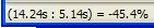 .
.
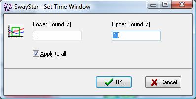
The alternative way to change the time window is to set the start and end points using the “change time window” icon in the tool bar. With this option all open data windows can be set to the same analysis times.

A third way to change the time window is to set it to triggered markers events- see section 5.4.6Settings, Trigger.
When the green frame surrounding the data analysis window is set so part of the beginning of the recording is not within the green frame (excluded from the analysis), that part of the x-y plot is shown in red and the rightward pointing green arrowhead on x-y plot moves to the point on the x-y plot where the analysis window begins. Likewise when the analysis window is set so part of the end of the recording is excluded this is marked in the x-y plot as yellow and the leftward pointing green arrow moves in the x-y plot to the new beginning of the data. This effect is illustrated below.
Up to 10 pairs of markers (Marker pairs 0 to 9) may be set on the time plots of roll and pitch. The beginning marker and end marker of each pair, as well as a label of the marker times are displayed.
 To select a marker
pair first click on the marker icon to obtain a pull down list of marker
pair possibilities. Once a pair is selected the beginning marker of the
pair can be placed at a location with a left mouse click, likewise the
end marker. When moving the vertical marker bar along the recording time
window, the time, roll and pitch angle and angular velocities at the marker
position are displayed in the lower status bar.
To select a marker
pair first click on the marker icon to obtain a pull down list of marker
pair possibilities. Once a pair is selected the beginning marker of the
pair can be placed at a location with a left mouse click, likewise the
end marker. When moving the vertical marker bar along the recording time
window, the time, roll and pitch angle and angular velocities at the marker
position are displayed in the lower status bar.
To remove a marker or all markers place the mouse on the marker so that marker symbol appears, click on the right mouse button and make an appropriate selection from delete marker pair or all markers.
Numerical values at the marker locations are listed under the tab “Marker Values” as shown below

For each marker pair the following information appears as marker values.
Marker begin and interval between markers
Roll and pitch angle amplitude and velocity at Begin and End Marker of the marker pair.
Difference in angle amplitude and velocity, as well as mean angular velocity between begin and end marker.
This information is also stored in the log csv file once the marker data has been stored.
The total recording duration is the time from the start to the end of the recording. It is not affected by changing the analysis time (green frame around the time histories) in the analysis window. The chosen duration is analysis time set by the green frame. It can be entered in the log file depending on the operation log file settings (see section 5.4.6).
Normal reference values are shown in the Data Analysis Window as triangles, thin vertical bars, and vertical rectangles next to the test subject’s values. The symbols are violet if the user assigned the reference value set to the recording. The triangles represent median values and the top and bottom of the vertical bars are equal to the 95 and 5 percentile limits, respectively and the top and bottom of the vertical rectangles are equal to the 75 and 25% percentile limits, respectively. These data are available for all the analysis variables listed above, except spectral densities and weights. Reference value sets are available for all pre-defined protocols in the standard balance deficit screening sequence.
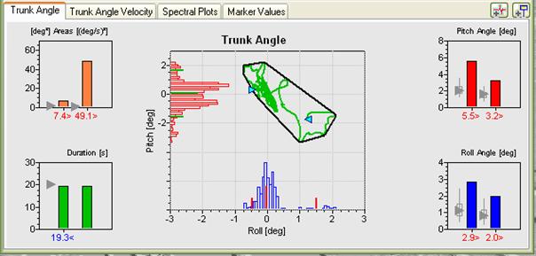
In the diagram above the pitch angle values of the patient standing eyes closed on foam are clearly above the 95 percentile limit but the roll values are on the edge of the 95 percentile. Consequently, the area values are also above the 95% limit. The duration is just shorter than normal (19.3 s) because the subject was not able to stand without falling for the maximum duration of the trial.
Displayed reference values are calculated for an age group ± 5 years either side of the test subject’s age (see diagonal yellow arrow above). There are at least 10 subjects in such age groups. If the subject’s values are greater than normal reference values, they are marked in red and followed by a >. If they are less, then they are marked in blue and followed by a <, otherwise in green and followed by a ~. Reference values are available for the ages 6 to 80 years. When no reference values are assigned, analysis values appear in white (black in printed versions) with no symbols following the value.
Note: Recordings should be long enough for reference values to be valid. Thus, reference values are considered applicable only if the duration of the recording is longer than 75% of the reference recording time.